Drawing an ASCII sketch
Every once in a while, I get a (seemingly) nice and interesting idea (thanks to a wonderful female creature, who’s always been my muse), and whenever I get one, I go straight to researching more about it, allocating most of my free time, so that I finish it up ASAP and show it to her. Last time, it was a CSS spewing thingy. This time, it was about generating an ASCII sketch of a picture.
I’m sure you’d have seen all those “Image to ASCII converter”, “ASCII art generator”, and all sorts of boring variants of this online. But, I’ll tell you where they all fail and how I managed to bring up a decent sketch in ASCII. It took me about 3 hours to come up with a basic sketch, and then a few more for making it more generic and deploying it in my website.
Mapping ASCII values over RGB…
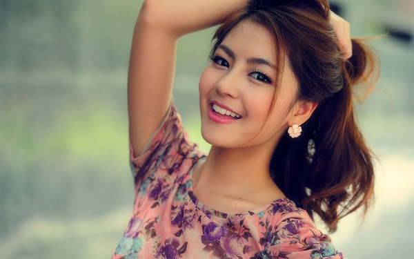
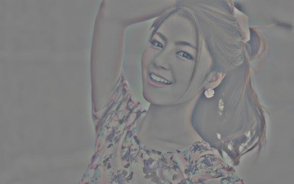
Let’s say I want to draw the ASCII sketch of this JPEG image…1
I always tend to hack on stuff with Python. And, it has an amazing image library to play with images. With PIL, we can do something like this,
>>> from PIL import Image
>>> img = Image.open('sample.jpg')
>>> px = img.load()
>>> px[0, 0]
(72, 94, 91)
So, we now have all those 3-tuple RGB values in a 2D array. The first step would be to convert these RGB values to intensities2 (i.e., grayscale, since the final ASCII art will look very similar to its grayscale version). It’s very easy, and PIL eases this a bit more,
>>> img = img.convert('L')
>>> px = img.load()
>>> px[0, 0]
87
Next stop is to have a bunch of characters sorted with respect to their pixel densities (like ' ' (space) for white, '.' (dot) for gray, '#' for black and so on), Once we have a character map, we simply map the characters over the grayscale image, like so…
>>> width, height = img.size
>>> for j in xrange(height):
...     print ''.join(CHARS[px[i, j] % len(CHARS)] for i in xrange(width))
Looks very simple, right? All we need to do is find CHARS (the character map).
There’s an ASCII art generator in Python, which has an interesting implementation for the character map. First, the printable ASCII characters are drawn in an image. Then, they’re sorted according to the pixel density of their render. This means, “space” has zero pixels, and so it will be the first thing you’ll find in the sorted list. Just what I wanted!
Let’s see how the ASCII image turns out after this mapping…
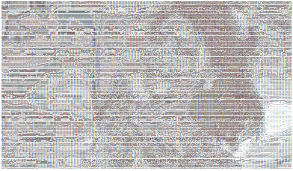
A gradient spew. Almost all the necessary details are gone! Bad luck, huh?
People work around this by clamping ranges of values to some character instead of using the entire ASCII table (like, all the colors ranging from light gray to white will be mapped to “space”). But, that’s still a workaround. It doesn’t help much.
Let’s see if we can tune this, by extracting necessary details from the image.
Getting the details…
An image (just like any other signal) can be represented as a sum of periodic (2D) waves of colors. It’s the magic of Fourier transform, that any signal can be represented as a sum of periodic waves of certain amplitudes and frequencies.
Let’s take our grayscale image and see how the first wave looks like,
>>> import numpy as np
>>> from numpy import fft as fourier
>>>
>>> ft = fourier.rfft2(img)         # get the 2D fourier transform of the grayscale image
>>> ft_new = np.zeros_like(ft)
>>> ft_new[0:1, 0:1] = ft[0:1, 0:1]
>>> rft = fourier.irfft2(ft_new)    # inverse transform
>>> img = Image.fromarray(rft)
>>> img.convert('L').save('fourier-1.jpg')
And, we get this - the initial component.

Now, let’s get the sum of first 3 waves…
>>> ft_new[0:3, 0:3] = ft[0:3, 0:3]     # we only need to change this line
>>> # everything else is the same
… and, we get the lowest frequencies from the image. This would be the base gradient.

… for 10 waves,
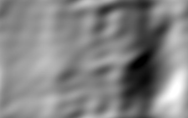
… and, for 50 waves,

Clearly, as we go further, the details are starting to show up. So, smaller frequencies indicate gradients, and higher frequencies indicate finer things. In other words, smaller frequencies tell you that there’s a face, whereas the higher frequencies show the finer details like edges, curvature, hairs, etc.
This means, we need the higher frequencies for the details. Well, we don’t have to fiddle around Fourier transform for achieving this, but it gives you an idea. Perhaps, the easiest way to get the details is by filtering out the lower frequencies.
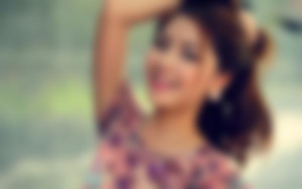
First, we blur the image. Let’s apply a Gaussian blur filter (I usually pick a radius of 7 or 8).
>>> from PIL import Image, ImageFilter
>>> img = Image.open('sample.jpg')
>>> blur_filter = ImageFilter.GaussianBlur(radius=8)
>>> blur_img = img.filter(blur_filter)
Since it’s a low pass filter, we get the image with the higher frequencies stripped out.
Now, we invert the image, and blend it with the original image (with 50% opacity)…
>>> from PIL import ImageOps
>>> inv_img = ImageOps.invert(blur_img)
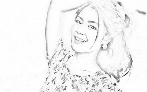
>>> blend = Image.blend(inv_img, img, 0.5)This leaves us with the details…
Now, we find a lot of gray areas. So, we have one last (and perhaps the important) step, which is to adjust the levels. For this, we move the image from RGB space to HSV space, clamp the levels to a certain minimum, maximum and gamma values, and convert it back to RGB.
You can think of this as making darker areas black and lighter areas white altogether! It’s quite simple. Here’s an answer from Stackoverflow that provides a Python implementation of how the levels are clamped.
As for our picture, once I clamp the levels (min = 78, max = 125, gamma = 0.78) and convert it to grayscale, I get this…
Looks like we’ve narrowed down more than enough details to get the ASCII art! Now, if we use the character mapping…
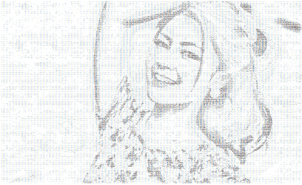
And, voila!
As a sidenote, you’re very welcome to play with my ASCII art generator, which does whatever I’d just shown you above.
See you next time!